
Volatility Regimes and Hidden Markov Models
The strategy reads a market regime off the volatility surface and sizes positions to it. This week the work was all on the first half — the regime read — and mostly about making it honest: moving it off a method that quietly used hindsight, widening what each regime is allowed to see, and starting a more ambitious model that lets the data decide how many regimes there are. None of it is finished. This is where it stood at the week's end.
What we're reading
The signal is the VIX and the shape of its term structure — the ratio of three-month to one-month implied volatility. In calm markets the curve is in contango (longer-dated above near-dated, ratio above 1); under stress it inverts into backwardation and the ratio drops below 1.
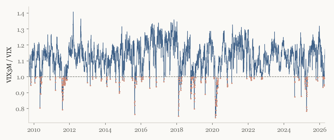
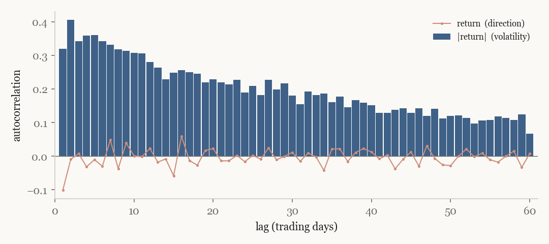
The reason a "regime" is a real object to model, and not just a label painted on afterwards, is that volatility persists. Calm follows calm; shocks arrive in bursts and take weeks to drain.
The model
A hidden Markov model assumes the market is in one of a few hidden states. We never see the state, only its emissions — returns and volatility features — and infer a probability over states from them. Three parts: the transitions (the chance of moving between states bar to bar), the emissions (what observations each state tends to produce), and the inference (how we turn observations into a state estimate). We use an input-output HMM, where the transition probabilities are themselves functions of the observed features, so the term structure actively pushes the model between regimes rather than transitions being fixed; the number of states is chosen by BIC, not set by hand. Most of this week was spent on the third part — inference — because that is where the dishonesty was hiding.
From hindsight to a causal filter
We had been reading the regime with a Viterbi decoding — the most-likely path of states given the entire history, future included. It decides early 2008 was a stress regime after watching the crash play out. That is fine for drawing a chart and ruinous for trading: every per-regime track record was built from labels no one could have had at the time. The concrete damage was in the sizing books. Because hindsight relabels the run-in to a crash as "stress," the calm-regime book never accumulated the crash days it had actually traded through — so it looked far cleaner, and got sized far larger, than it deserved.
We replaced Viterbi with a causal forward filter: at each bar it returns the probability of each state using only data up to that bar, lag and all, and we rebuilt the per-regime sizing books from the labels it produced live. The honest books changed the bet. Where the hindsight version had wanted tens of times leverage on regimes that looked spotless, the live-history version settled to a few times, with no artificial caps — because the books now carry the messy days the hindsight labels had quietly removed.
Widening what a regime sees
Next, what defines a regime. It had been the size of the day's return alone — big down-days one state, quiet days another. We widened the emissions to multivariate, so a regime is defined by market conditions (the term structure and related features), not just the magnitude of the move. The first real run of this, across 2015–2018, was a mess, and it is worth recording as one rather than tidying away:
| First multivariate run, 2015–2018 | What we saw |
|---|---|
| number of regimes (BIC, per refit) | unstable — flips between 2 and 5 |
| neural-context validation accuracy | 9% to 100% by window — an uninformative metric (overlapping samples) |
| per-regime sizing | some stress regimes came out wanting long bets — labels carried over from the wrong state |
| regime labels | no longer interpretable once the emissions are multivariate |
None of these is fatal, but together they say the wider model is doing something we do not yet understand or trust; two of the diagnostics turned out to be measuring artifacts rather than signal. Logged, and left for the stress-testing that has to come before any of it is believed.
The lag, and the two things aimed at it
Why push past a working rule-based version at all? Because the rule-based read is late. A threshold on today's term structure misses a regime that builds slowly — thirty quiet down-days in a row, each unremarkable alone. That lateness is not academic: an early build of the strategy carried it into a roughly −94% drawdown in the first quarter of 2026, sitting in the wrong regime straight through a turn.
Two responses went on the board. The first is a small Transformer that reads a multi-month window and compresses it into the HMM's transition inputs, so a slow build-up can register before any single day trips a threshold; it is designed and started, not yet trained. The second is a different model entirely.
Letting the data choose the regimes
The most ambitious build of the week: a sticky hierarchical Dirichlet process HMM — a nonparametric model that, instead of taking the number of regimes as given, infers it, with a built-in "sticky" preference for regimes that persist rather than flicker. The appeal is obvious: stop hand-picking how many market states exist and let the data say. The cost is the inference — it is fit by Gibbs sampling rather than solved, and samplers for models like this are temperamental. The first smoke test ran end to end on 2008 data, but immediately pushed against its own ceiling on the number of states and let its persistence parameter swing high. It runs. Whether it works is exactly the question the week ended without answering.
| Regime read | what it is | status at week's end |
|---|---|---|
| rule-based | hand-set term-structure thresholds | the baseline to beat — reliable, but late on turns |
| forward filter (was Viterbi) | state probabilities from past data only | adopted; replaced the hindsight labelling |
| multivariate emissions | regimes defined by conditions, not return size | built; first run not yet trustworthy |
| Transformer context | summarise a multi-month window into the inputs | designed, not trained |
| sticky HDP-HMM | infers the number of regimes itself | runs; unproven |
Sizing
The regime read is half the system; the bet is the other half. We keep a per-regime Kelly book — each regime accrues its own live track record, and the bet scales with that regime's edge, run at a fraction of full Kelly. The causal-filter change is what makes this honest, because the books are now built from labels that were knowable at the time. The standing constraint, which shapes most of what follows, is that a regime has to hold its identity across refits for its book to mean anything — and the model that picks its own number of regimes is the one most likely to strain that.
Where it stands
The regime read is causal and the sizing honest; the emissions are wider but not yet trustworthy; a slow-build detector is sketched; and the model that chooses its own number of regimes runs but is unproven. The next job is the obvious one and the hard one: stop adding pieces and stress-test the most ambitious of them, to find out whether it has learned anything or only looks as though it has.