
The Fancy Model Lost
This is a working log of what we ran this week, in order, with what each test returned. Going in, the model is an input-driven hidden Markov model with Gaussian emissions and a single regime feature — a volatility term-structure signal. On the late-2018 test window it produces five regimes, three of which pass a trust check (their edge keeps its sign across sub-periods) and two of which don't. The week's question was narrow: does adding capacity beat that? We ran six things. Most of the durable progress came from the least glamorous of them.
1. A switching dynamical system
Ran it because the HMM holds the dynamics fixed inside a regime, and we wanted to let a regime drift — to model a slow deterioration rather than only "calm" or "stressed". This is the most capable model we tried all week.
It fought us before it told us anything. The maintained, easy-to-install library only had the plain version, without the input-driven switching we specifically wanted to test; the library that had it needed a heavy compiled toolchain and source patches just to build. Once running, the input-driven version diverged numerically — its objective ran off into the 1e17–1e19 range, and neither clipping the inputs nor penalising the weights settled it. A build-up test pinned the blow-up to the moment the inputs were added; the plain Markov version fit cleanly on the same data. The only way to get a result was to switch off the input-driven part — the part under test.
Stripped to what would run, it scored 0 of 5 trustworthy regimes against the baseline's 3, collapsing into two near-identical regimes (52% and 40% of the data with almost the same mean) because it had nothing left to tell them apart. The honest conclusion is not "it lost" so much as "we couldn't run the comparison we wanted." Parked, not killed.
2. Student-t emissions
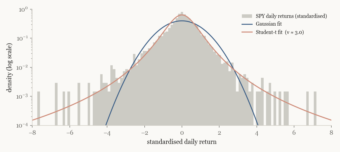
Back inside the working framework. Returns inside a regime have far heavier tails than a Gaussian allows; this had been tried on an older model line but never on the current one, so it was a real untested lever. We built it from scratch — diagonal Student-t emissions with a tail-heaviness parameter, ν, learned per regime from the data (the standard scale-mixture EM of Peel & McLachlan, 2000, with ν found by a one-dimensional root solve over its natural range).
On the test window it gave the same 3-of-5 trustworthy count — it didn't change which regimes pass — but the passing regimes scored higher. The part worth keeping was ν itself: the extreme regimes learned ν ≈ 3 (heavy-tailed), the calm middle regimes pinned at the Gaussian end. We didn't tell it which regimes are dangerous; it worked that out.
3. A trust metric that survives sampling noise
A smaller build, because the trust check underneath everything else needed it. The problem: regimes were being judged partly on how stable their Sharpe is across sub-periods, but Sharpe is noisy, and that noise looks like instability. We built a metric that subtracts the expected sampling noise (the Lo, 2002, standard-error envelope for a Sharpe ratio) from the observed spread and keeps only what's left. The first version had a units error that inflated the noise term roughly 500× — caught by sanity-checking it against magnitudes we expected. Every "trustworthy regime" count in this post runs through the corrected gate.
4. Brute force vs the greedy search
The model picks its number of regimes with a greedy procedure that splits and merges states as it goes. Worth checking whether it actually finds the best count, so we built a plain version that just sweeps every count from 2 to 10 under the identical penalty. The sweep found a strictly better-scoring fit at 7 regimes than the greedy procedure's 5 — the greedy search had settled into a worse local optimum. But more regimes isn't free: each one gets fewer bars, so the trust check has less to work with per regime.
| Search | regimes | trustworthy | note |
|---|---|---|---|
| greedy, Gaussian | 5 | 3 | the incumbent |
| greedy, Student-t | 5 | 3 | stronger passing regimes |
| exhaustive, Gaussian | 7 | 4 | finer carve of the signal |
| exhaustive, Student-t | 7 | 5 | most trustworthy, thinnest regimes |
More trustworthy regimes from the exhaustive Student-t, but each is built on half the data. Neither is strictly better; we left both on the table rather than declare a winner.
5. The bug that erased last week's result
Wiring up the per-regime statistics, we found a same-day look-ahead: a bar was being labelled with the regime read that included that bar's own data, then paired with that same bar's return — so the position was, in effect, chosen already knowing the outcome. It had inflated per-regime Sharpe about 3× and the implied leverage 3–10×.
Fixing it — label each bar with the forecast regime, the one knowable before the bar — turned the previous week's headline into a loss. That "+11.66%, Sharpe +0.87" on an earlier model, and the whole story we'd built around it, was the bug; with the forecast labelling, all four of those older variants underperform buy-and-hold by 0.4–6%. The result we'd been pleased with seven days earlier did not exist.
To make sure the fix was itself clean, we built a sandbox that physically deletes every future bar before each prediction and re-runs. The first attempts differed from the live pipeline at the 1e-3 level — which turned out to be burn-in and date-boundary conventions in the test, not leaks in the model — and once reconciled it matched to the last decimal, 0.00e+00. That bit-exact match is the bar we now hold any "is this causal?" claim to.
6. The clean result, and whether it travels
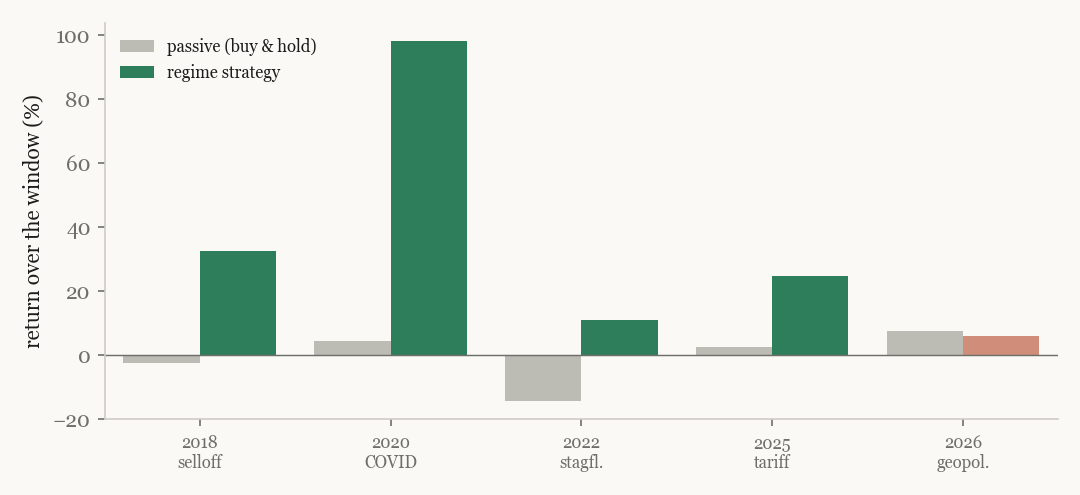
With the fix in, the model's per-regime bet on the test window is genuinely two-sided — it shorts through the selloff and goes long into the recovery — and beats passive by 35–65 points across the variants. Out of sample on five historical windows it was profitable in all five and beat buy-and-hold in four:
One caveat we kept attached to this result: the thing that actually made the difference was the feature, not the model class. The current single feature has several times the standalone separating power of the older ones we used to feed the model; swap it back and the cleverest architecture still fails. It is mostly about what you feed the regime model, not which regime model you use.
7. Sizing: raw Kelly is untradeable
The per-regime Kelly bet the model wants is enormous, precisely because the regimes are so distinct — full Kelly asks for tens of times leverage, regime by regime.
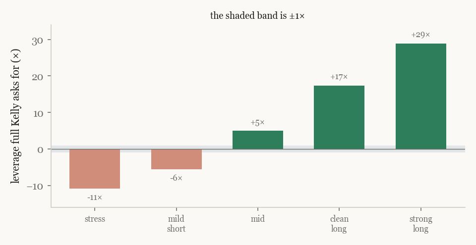
We had been hard-clipping to ±1, which on 82–99% of bars just pins the bet at the limit — it throws away the gradation and bets the sign at full size. Replacing the clip with a fixed fraction of Kelly (no cap) kept the gradation — typical bet 0.5–3×, median about 1× — and beat the clip on every metric across the five windows.
| Sizing | mean return | Sharpe | worst drawdown |
|---|---|---|---|
| hard clip to ±1 | +34.4% | +1.47 | −11.5% |
| fixed fraction of Kelly | +52.7% | +2.01 | −8.2% |
The one thing the more aggressive gradation did was tip the 2026 geopolitical window from a small gain to a small loss — sharpening, not causing, the failure we already had there.
8. The clever sizing that did nothing
We also built a "quality-weighted" Kelly — scale each regime's bet by a combined trust-and-Sortino score. On the clipped sizing it looked like a +20-point improvement; under fractional Kelly it was a no-op. The lift had been the clip's, not the idea's: once the bet isn't being clipped, the weighting cancels algebraically wherever the model is confident. Built, tested, reported flat, parked.
Where that leaves the week
Not a tidy story. The most capable model is parked unresolved rather than beaten; the gains that stuck were a heavier-tailed emission and a fraction-of-Kelly bet; the single biggest correction was a bug fix that deleted the prior week's headline; and one window still defeats the whole thing. "The fancy model lost" is too clean — nearer the truth is that we couldn't run the fancy model the way we wanted, the plain changes paid and the clever ones mostly didn't, and what really moves this system is the feature it reads, not the machinery around it. Next week goes at the window that beat us.