
No Arbitrary Rules
Last week we stripped the inherited model back to a single-feature emission to get its sampler moving. It worked, but the choice was arbitrary — a scalar emission is no more "the model the data justifies" than a seven-feature one. So this week opened by turning that discomfort into a rule, and then spent itself letting measurements, rather than arguments, decide what to build. The result is not where we expected: the working model is the plainest thing on the table, not the most elaborate.
The rule
We wrote down the principle we'd violated and the habits it bans. The rule: build the model the data justifies, not the model that is easy to read. In practice it forbids three moves we kept reaching for while debugging:
- Don't thin the features to make the likelihood behave. If a model misfits in
many dimensions, the fix is the distribution, not deleting the dimensions that carry the regime information.
- Don't add a knob to pin the number of regimes. The model's own prior is the
correct statement of how many states the data supports; a penalty that forces a tidy count is a preference smuggled in as code.
- Don't switch a component off to make a chart look clean. Disabling a piece to
debug another is a temporary diagnostic, never a fix.
Behind all three is one rule that governed the rest of the week: a healthy diagnostic is not a correct model. A sampler that mixes, a state count that settles, a parameter that lands on a sensible value — all necessary, none sufficient.
The principled fix we dropped
The honest answer to last week's dimensionality problem was not to delete features but to change the emission distribution: swap the Gaussian for a heavier-tailed Student-t, so a point in the "wilderness" between states is unlikely rather than impossible, and the sampler can move. We built it — per-state tails, learned from the data — and it worked in the right direction: on the frozen window the emission gap fell about 30%. Not enough to unfreeze the chain, and, more to the point, we caught ourselves optimising the wrong thing. The emission gap is a number inside the sampler; the strategy's job is to read regimes in time to size down before a shock and back up into a recovery. Whether the chain prefers three states or twelve is irrelevant if three detect the shock fast enough. We paused the emission work — the implementation is sound and kept — rather than tune a proxy for its own sake.
A scorecard for the actual job, and a fast way to run it
So we built the scorecard the work actually needed. Mark each day from price alone: a "shock" day is one trading well below its recent high, a "calm" day one barely off it. Then ask how often the model has left its baseline state on the shock days and how often it sits in baseline on the calm days, and average the two. Fifty per cent is a coin flip. It rewards being in the right kind of state at the right time and nothing else.
To run that over and over we built a replay harness: fit a model once on history up to the eve of a known episode, freeze it, and forward-filter through the episode one bar at a time. A run that took hours now takes seconds, and fits are cached. The first thing it caught was a bug worth recording: on an early smoke test the model switched state 187 times in 188 days. It had quietly memorised the time of day — every morning bar to one state, every afternoon bar to another — because those features sat in the emission and split the data cleanly. A model with a perfectly healthy-looking fit that was reading the clock. Moving the time features out of the emission and into the transitions fixed it: three switches instead of 187. Exactly the "healthy diagnostic, wrong model" trap the rule was written for.
Letting the data pick the architecture
With a fast loop and an honest metric, the architecture question stopped being a debate. The first cut put the elaborate inherited model — the nonparametric HDP-HMM we'd spent two weeks on — against a plain input-output HMM and the hand-coded rules. The inherited model came last: never above 61%, too sticky to move off baseline. The plain IO-HMM won outright, catching 94% of the COVID shock days while still returning most calm days to baseline. So the working model pivoted off the inherited one. Then the fuller bake-off, four architectures on three windows, one metric:
| Model | late 2018 | COVID 2020 | 2022 grind | mean |
|---|---|---|---|---|
| hand-coded rulebook | 50.0 | 49.9 | 67.3 | 55.7 |
| IO-HMM (frozen) | 75.5 | 81.5 | 61.8 | 72.9 |
| nonparametric (truncated HDP) | 57.0 | 57.7 | 51.6 | 55.4 |
| split-merge IO-HMM | 78.8 | 81.5 | 61.8 | 74.1 |
Balanced accuracy, percent; 50 is chance. The two input-output HMMs win clearly. We adopted the split-merge variant — narrowly ahead of the frozen one on 2018 and otherwise tied, and it gives flexibility in the state count for free if richer emissions ever justify it. One honesty note: the nonparametric model's row is not a fair verdict on it. A default pruning threshold meant its sparsity mechanism never actually engaged, so that 55% is a statement about one hyperparameter, not about the approach. We logged it as inconclusive, not as a loss.
Why everything collapses to two regimes
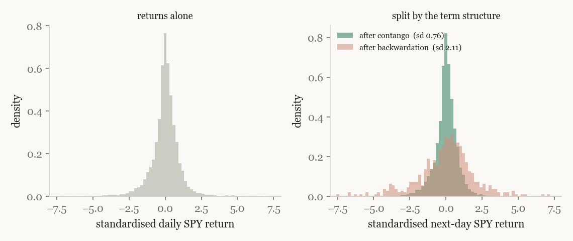
The awkward finding underneath the table: every learned model picks two states. Not by accident — it's structural. Adding a third regime costs the model-selection penalty far more than the fit it buys (a few hundred nats of penalty against about a dozen of likelihood), and the input-driven transition matrix grows with the square of the state count, which makes it worse. Even on synthetic data with four regimes planted by hand, it picks two. So the lever for richer regime structure is not the architecture and not the state-count search — it is the emission, what each state is allowed to see. On returns alone, two regimes is all there is.
What it does, and doesn't, do
Two honest limits to close on. First, the rules still beat the learned models on the slow 2022 grind (67.3 vs 61.8) — because the rules read the term structure directly, while the HMM emits on returns only and a small persistent drift looks like calm to a return-only Gaussian. That is an emission-feature gap, not an architecture failure, and it points the same way as everything above. Second, we tested the model as an actual forecaster — predict tomorrow's direction — and it sits at a coin flip:
| Window | model sign accuracy | always-up baseline |
|---|---|---|
| late 2018 | 53.5% | 51.2% |
| COVID 2020 | 52.3% | 56.5% |
| 2022 grind | 48.2% | 48.8% |
Around 50.6% on aggregate, inside the sampling noise. The model is a regime labeler, not a direction forecaster — which is fine for sizing, where being in the right state matters more than calling the next day's sign, but should not be dressed up as prediction.
The week leaves two results side by side: an architecture chosen by measurement rather than argument — and the plainest one, not the inherited showpiece — and a frank account of how little returns alone contain. Both point the next work at the same place, the emission: put the term structure back into what each state sees, carefully, at a dimensionality the model can survive. Which is exactly where the inherited model went wrong by overloading it.